This chapter documents the insertion of static figures, the generation of figures from Python code, multi-column layout, and the special case of PDF-only figures (TikZ, PGFplots).
The identifier #fig-label allows a cross-reference with @fig-label. The width attribute accepts percentages or absolute values (5cm, 0.5\linewidth).
Here is an example with the cnam logo:
{#fig-logo-cnam width=40%}
Figure 2.1: The official cnam logo.
Figure 2.1 shows the official cnam logo, loaded from the images/ folder at the project root.
AstuceRecommended image formats
PDF: prefer vector formats .pdf or .eps for diagrams and charts (sharp at all resolutions). For photographs, .png or .jpg at 300 dpi minimum.
HTML: all standard web formats (.png, .jpg, .svg). .svg files are particularly well suited for diagrams.
Quarto automatically handles format conversion depending on the render target.
AvertissementPaths are relative to the .qmd file, not to the project root
Image paths are relative to the location of the .qmd file. From content_en/chapters/, the images/ folder at the project root is at ../../images/myfile.png. This behaviour is identical in PDF and HTML.
2.2 Python-generated figures
Quarto can execute Python cells (via Jupyter) and include their graphical output as numbered figures. The chunk syntax uses options prefixed with #|:
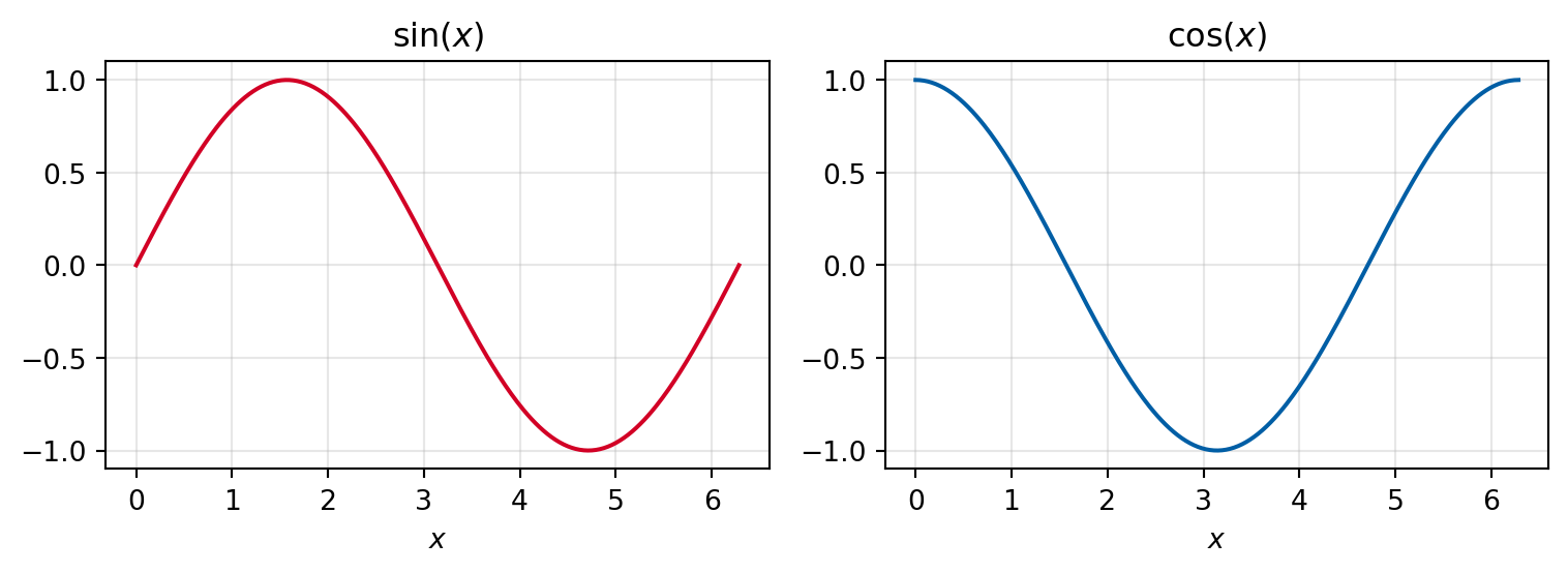
```{python}#| label: fig-sincos#| fig-cap: "Curves $\\sin(x)$ and $\\cos(x)$ over $[0, 2\\pi]$."#| echo: trueimport numpy as npimport matplotlib.pyplot as pltx = np.linspace(0, 2* np.pi, 300)fig, axes = plt.subplots(1, 2, figsize=(8, 3))axes[0].plot(x, np.sin(x), color='#d20025')axes[0].set_title(r'$\sin(x)$')axes[1].plot(x, np.cos(x), color='#005EA5')axes[1].set_title(r'$\cos(x)$')for ax in axes: ax.set_xlabel('$x$') ax.grid(True, alpha=0.3)plt.tight_layout()```
Output:
import numpy as npimport matplotlib.pyplot as pltx = np.linspace(0, 2* np.pi, 300)fig, axes = plt.subplots(1, 2, figsize=(8, 3))axes[0].plot(x, np.sin(x), color='#d20025')axes[0].set_title(r'$\sin(x)$')axes[1].plot(x, np.cos(x), color='#005EA5')axes[1].set_title(r'$\cos(x)$')for ax in axes: ax.set_xlabel('$x$') ax.grid(True, alpha=0.3)plt.tight_layout()
Figure 2.2: Curves \sin(x) and \cos(x) over [0, 2\pi].
Figure 2.2 is generated at each compilation. With execute: freeze: auto in _quarto.yml, Quarto caches the results in _freeze/ and only re-executes the code if the chunk has changed — useful for figures that take a long time to compute.
Avertissementplt.tight_layout() is essential
Without plt.tight_layout(), axis labels frequently overlap in the PDF. Always end your matplotlib figures with this line.
Astuceecho: false for the final document
During writing, echo: true displays the code — convenient for review. For the version submitted to the doctoral school, switch figure chunks to #| echo: false to display only the graphic.
2.3 Multi-column layout
The layout-ncol directive places several figures side by side. Apply it to a div containing sub-figures:
Some complex figures can only be generated in LaTeX (TikZ, PGFplots, circuitikz…). They are inserted via a {=latex} block inside a figure div, accompanied by replacement content visible in HTML:
:::{#fig-tikz fig-pos='h'}```{=latex}\centering\begin{tikzpicture} \draw[thick, ->] (0,0) -- (3,0) node[right] {$x$}; \draw[thick, ->] (0,0) -- (0,2) node[above] {$y$}; \draw[blue, thick] plot[domain=0:2.8, samples=50] (\x, {sin(\x r)});\end{tikzpicture}```::: {.content-visible when-format="html"}*(TikZ figure — available in the PDF version only)*:::Example TikZ figure inserted as raw LaTeX.:::
Output:
(TikZ figure — available in the PDF version only)
Figure 2.4: Example TikZ figure inserted as raw LaTeX.
AstuceAlternative: compile the TikZ figure as a separate PDF
For complex TikZ figures, a more robust approach is to compile them as a standalone .pdf file, then include them as a regular image:
This avoids package conflicts and speeds up compilation.
2.5 Float positioning (PDF)
In LaTeX, figures and tables are floats: LaTeX decides their position to achieve the best possible layout. The fig-pos attribute (figures) or tbl-pos (tables) allows you to give it instructions.
Forces placement here, without any floating (requires \usepackage{float})
The default value in Quarto is tbp. For a Python chunk, the specifier is passed as a cell option:
```{python}#| label: fig-python#| fig-cap: "My figure."#| fig-pos: 'h'```
To set a default specifier for the entire document, add to _quarto.yml:
fig-pos:'H'
Avertissementh is not a guarantee
The h specifier asks LaTeX to place the float here if possible, but LaTeX may ignore it if there is insufficient space. The combination ht (here, then top of page) is generally more robust. H forces placement unconditionally, but can create nearly empty pages if the figure is large — reserve it for cases where position is truly critical.
NoteFloats only apply to PDF
In HTML, fig-pos and tbl-pos are ignored: figures and tables are inserted in the document flow at their insertion point, like any other element.